Non-linear mechanical field reconstruction coupling recurrent neural networks with physics-informed graph neural networks

Abstract

Reconstructing local stress fields in heterogeneous microstructures under non-linear, history-dependent loading remains a major computational bottleneck in multi-scale simulations. We propose a coupled LSTM-GNN framework that links the temporal and spatial aspects of local stress field reconstruction. A Long Short-Term Memory network encodes macroscopic stress-strain sequences into a compact hidden state that captures the path-dependent constitutive response, while a physics-informed Graph Neural Network reconstructs the spatially-resolved stress field at each time step. We introduce a relative weighting strategy with linear warm-up to balance the data-driven reconstruction loss and a discrete divergence-based equilibrium penalty. This resolves the scale mismatch that prevents fixed-weight formulations from converging in the elasto-plastic regime.

The model is trained on 10,000 non-proportional loading paths applied to a periodic plate-with-a-hole microstructure and von Mises elasto-plasticity. The model achieves three orders of magnitude speedup over finite element simulations and generalizes to loading sequences twice the training length, with 1.9% cumulative error. Because the graph relies on mesh connectivity instead of the specific element type, one trained surrogate can be applied directly without retraining to meshes with different element types and to both coarser and finer resolutions, while in all cases reproducing the high-fidelity quad-element FE field used during training. Indeed, the message passing characteristics inherent to GNN and MeshGraphNet architecture render the model mesh-agnostic. Analysis of the LSTM hidden states suggests a low-dimensional structure related to the internal state variables of the constitutive model.

Graph neural networks
Multi-scale simulation
Recurrent neural networks
Machine learning
Architectured materials
Local stress field reconstruction
Physics-informed neural networks

Method

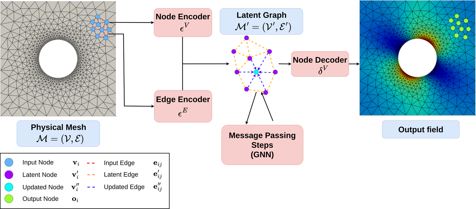
The surrogate splits the problem in two. An LSTM reads the macroscopic stress-strain history and compresses it into a hidden state that encodes the path-dependent response. A graph neural network then takes that hidden state as a node feature and performs message passing over the mesh to localize the full stress field, one step at a time. A divergence-based penalty pushes the predicted field toward mechanical equilibrium.

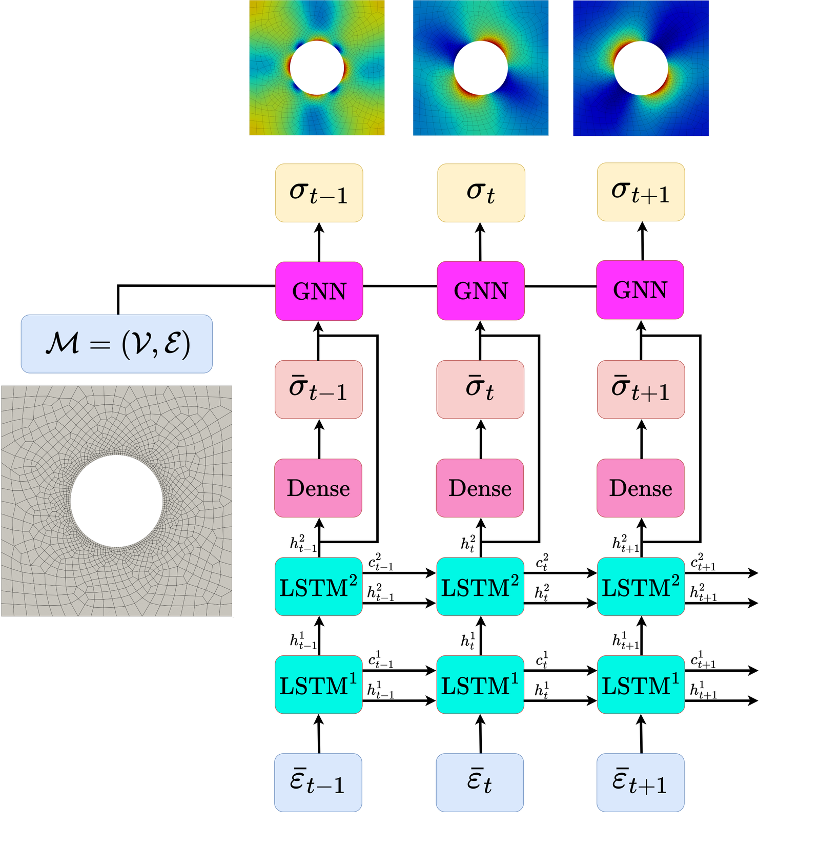
Coupled LSTM-GNN architecture — **Coupled architecture.** The LSTM processes the mean strain history to produce hidden states and mean-stress predictions; these become enriched node features for the GNN, which reconstructs the local stress field on the periodic mesh graph at each time step.

The two networks are chained explicitly. At each step $t$, the LSTM maps the macroscopic strain and its previous hidden and cell states to the mean stress and the updated states:

$$\mathrm{LSTM}\!\left(\bar{\boldsymbol{\varepsilon}}_t,\, \boldsymbol{h}^{2}_{t-1},\, \boldsymbol{c}^{2}_{t-1}\right) \;\longmapsto\; \left(\bar{\boldsymbol{\sigma}}_t,\, \boldsymbol{h}^{2}_t,\, \boldsymbol{c}^{2}_t\right)$$

The mean stress $\bar{\boldsymbol{\sigma}}_t$ and hidden state $\boldsymbol{h}_t$ are broadcast to every node and concatenated with its coordinates $\mathbf{x}_i$ and boundary label $\alpha_i$ to form the node features:

$$\boldsymbol{v}_{i,t} = \left(\bar{\boldsymbol{\sigma}}_t,\, \boldsymbol{h}_t,\, \mathbf{x}_i,\, \alpha_i\right)$$

The GNN then reconstructs the three local stress components at each node of the mesh $\mathcal{M}$:

$$\mathrm{GNN}\!\left(\bar{\boldsymbol{\sigma}}_t,\, \boldsymbol{h}_t,\, \boldsymbol{v}_{i,t},\, \mathcal{M}\right) \;\longmapsto\; \left(\sigma_{xx_{i,t}},\, \sigma_{yy_{i,t}},\, \sigma_{xy_{i,t}}\right)$$

Composing the two yields a single end-to-end map from the loading history to the local stress field:

$$\mathrm{GNN}\!\left(\mathrm{LSTM}(\bar{\boldsymbol{\varepsilon}}_t,\, \boldsymbol{h}_{t-1}),\, \boldsymbol{v}_{i,t},\, \mathcal{M}\right) \;\longmapsto\; \left(\sigma_{xx_{i,t}},\, \sigma_{yy_{i,t}},\, \sigma_{xy_{i,t}}\right)$$

GNN architecture — **Spatial decoder.** An encode–process–decode GNN maps the mesh to a latent graph, runs message passing, and decodes the local stress field.

Physics-informed loss

The reconstruction is trained with a normalized mean squared error that weights each of the $d$ stress components equally:

$$\mathrm{NMSE}(\boldsymbol{\sigma}, \hat{\boldsymbol{\sigma}}) = \frac{1}{d}\sum_{c=1}^{d} \frac{\sum_{i=1}^{n}\left(\sigma_{c,i}-\hat{\sigma}_{c,i}\right)^2}{\sum_{i=1}^{n}\left(\sigma_{c,i}-\frac{1}{n}\sum_{j=1}^{n}\sigma_{c,j}\right)^2}$$

A discrete divergence penalty drives the predicted field toward mechanical equilibrium, $\mathbf{div}(\boldsymbol{\sigma})=\mathbf{0}$, evaluated at the interior nodes:

$$\mathcal{L}_{\mathrm{div}} = \bigl(\mathbf{div}(\hat{\boldsymbol{\sigma}})\bigr)^2 = \frac{1}{n}\sum_{i=1}^{n}\left\|\,\mathbf{div}(\hat{\boldsymbol{\sigma}})\big|_{\mathbf{x}=\mathbf{x}_i}\right\|^2$$

The two terms differ by orders of magnitude, so a fixed weight fails. A relative weighting with linear warm-up keeps the physics penalty at a controlled fraction of the gradient, regardless of absolute scales:

$$\mathcal{L}_{\mathrm{total}} = \mathrm{NMSE} + \lambda_{\mathrm{eff}}\,\mathcal{L}_{\mathrm{div}}, \qquad \lambda_{\mathrm{eff}} = \lambda_{\mathrm{rel}}\, w(e)\, \frac{\overline{\mathrm{NMSE}}}{\overline{\mathcal{L}}_{\mathrm{div}} + \varepsilon}$$

with the warm-up $w(e) = \min(1,\, e/K)$ over $K$ epochs. We use $\lambda_{\mathrm{rel}} = 0.1$ and $K = 20$, so the penalty reaches about 10% of the total loss after warm-up.

Training convergence. Validation NMSE over 100 epochs. Adding the divergence penalty does not degrade reconstruction — P-DivGNN matches or improves on the baseline GNN.

Results

Macroscopic stress-strain response

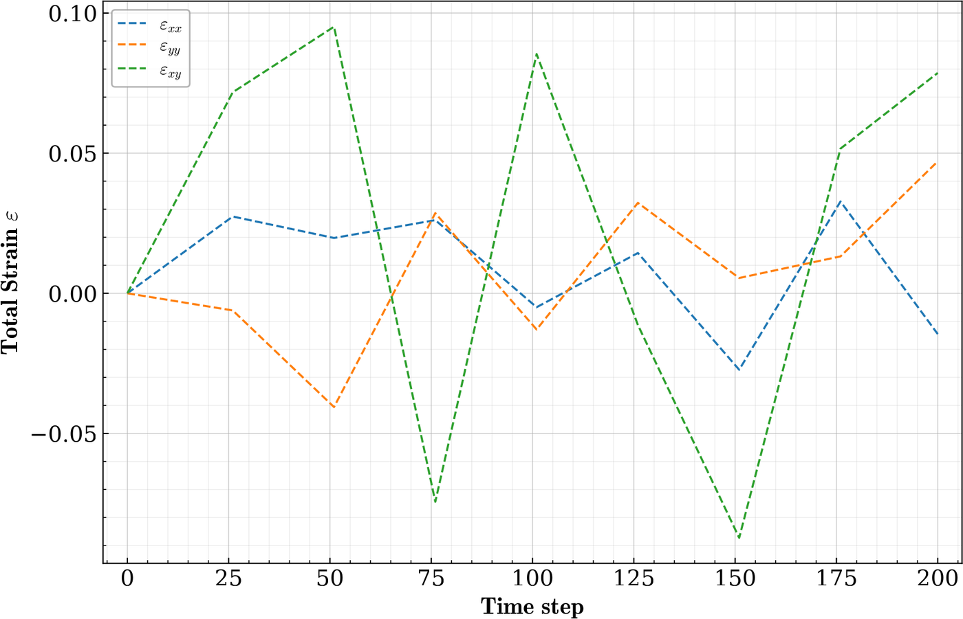
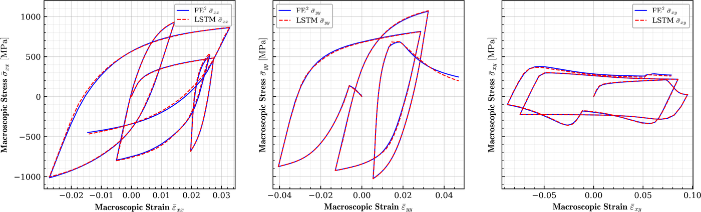
Given an input strain path, the LSTM predicts the macroscopic stress response. On this eight-segment path — twice as long as those seen during training — it tracks the finite-element reference with 1.9% cumulative error.

Input macroscopic strain path — **Input.** A non-proportional, eight-segment macroscopic strain path.

LSTM macroscopic stress-strain response — **Response.** Macroscopic stress-strain curves per component: the LSTM (dashed) reproduces the finite-element reference (solid) across every hysteresis loop.

FE vs. surrogate — drag to compare

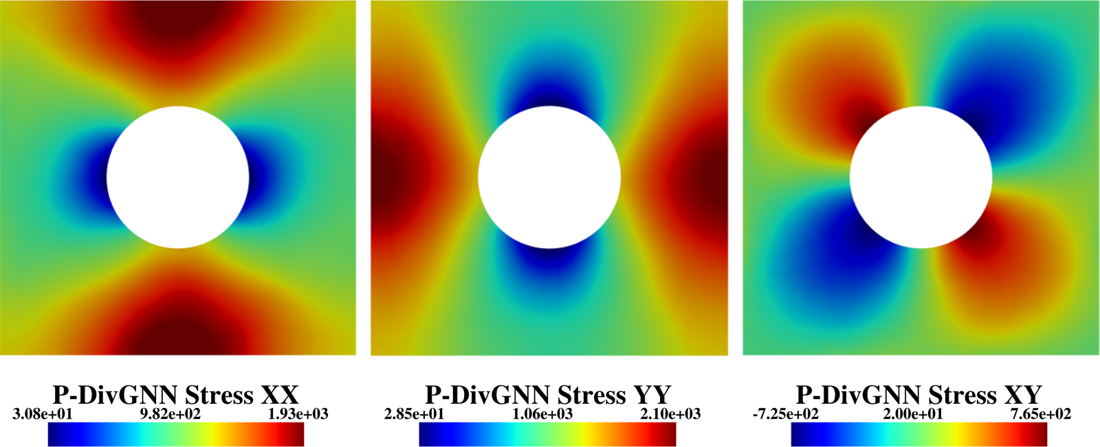
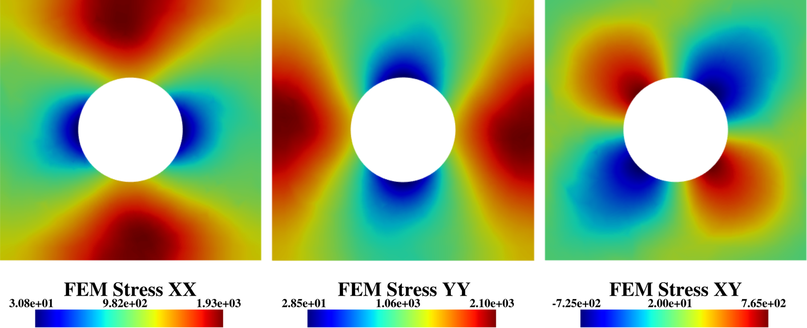
Final-step stress field (σ_xx, σ_yy, σ_xy), shared color scale. Drag the handle: finite-element reference on the left, the surrogate on the right. Toggle which surrogate to compare against.

↔

FE (reference) P-DivGNN

Divergence field

The clip plays the full loading path, showing the stress divergence for the finite-element reference, the baseline GNN, and the physics-informed P-DivGNN. The divergence penalty visibly drives the surrogate toward equilibrium.

Stress divergence along the loading path: FE, GNN, and P-DivGNN (lower is closer to equilibrium).

One model, any mesh

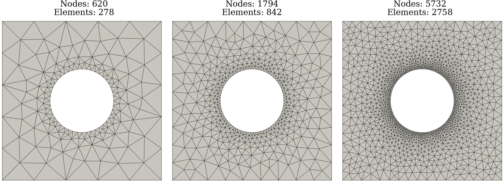
The same trained surrogate — never retrained — is evaluated on coarse, medium and fine triangular meshes. Switch between the finite-element reference and the surrogates.

Mesh refinement levels — Coarse · medium · fine. The graph depends on mesh connectivity, not element type, so a single surrogate transfers across resolutions while reproducing the high-fidelity FE field.

LSTM hidden-state analysis

The LSTM compresses the loading history into a 64-dimensional hidden state. Reduced to 2D with PCA and t-SNE, the per-step states trace a low-dimensional path that mirrors the loading. Drag the slider (or press play) to follow the eight-segment loading path used in the paper (twice the training length): the red line marks the current step on the strain path, and the highlighted point shows where that step sits in each embedding. Points are colored from the start (dark) to the end (yellow) of the path.

Eight-segment strain path (ε_xx, ε_yy, ε_xy) — red line = current step

PCA of the hidden states

t-SNE of the hidden states

step 0

Performance

3,500×

faster than finite elements at >50k nodes

< 0.2 s

per RVE — real-time field reconstruction

1.9%

cumulative error at twice the training sequence length

Inference time vs. mesh size

GPU neural-network inference (NVIDIA RTX A4000, 16 GB) vs. CPU finite-element solving (Intel Xeon W5-2455X). The GNN scales linearly with the number of nodes; the LSTM cost is essentially constant.

The physics-informed weighting lowers the overall NMSE from 1.68×10⁻² (GNN) to 1.56×10⁻² (P-DivGNN, −7%) and cuts the mean stress divergence from 893 to 440 (−51%), at an overall macroscopic wMAPE of 1.22%.

Highlights

Trained on a fine mesh, the surrogate predicts high-fidelity fields on coarse meshes.
Divergence-based physics penalty enforces equilibrium with automatic loss balancing.
LSTM-GNN coupling predicts a single RVE in real time, up to 3,500× faster than FE.
Accurate on loading paths twice as long as those seen during training.

Citation

M. R. Guevara Garban, Y. Chemisky, É. Prulière, M. Clément, M. Abendroth, B. Kiefer. Non-linear mechanical field reconstruction coupling recurrent neural networks with physics-informed graph neural networks. arXiv:2606.10909 [cs.CE], 2026. Submitted to Computer Methods in Applied Mechanics and Engineering.

@article{GuevaraGarban2026LSTMGNN,
  author  = {Guevara Garban, Manuel Ricardo and Chemisky, Yves and
             Pruli{\`e}re, {\'E}tienne and Cl{\'e}ment, Micha{\"e}l and
             Abendroth, Martin and Kiefer, Bjoern},
  title   = {Non-linear mechanical field reconstruction coupling recurrent
             neural networks with physics-informed graph neural networks},
  journal       = {Computer Methods in Applied Mechanics and Engineering},
  year          = {2026},
  eprint        = {2606.10909},
  archivePrefix = {arXiv},
  primaryClass  = {cs.CE},
  note          = {Submitted; preprint arXiv:2606.10909}
}